[paper] Transformer 실습을 통해 익히는 Pytorch 기초 (Attention is All you Need)

728x90

Transformer 이전 (RNN LSTM)

Naive sequence model

t-1, t-2..........1 를 고려한 xt의 확률

이전 데이터들을 전부 고려해서 다음을 찾는 방식

(초기는 할만한데 이후로는 너무 정보가 늘어난다)

Naive sequence model -> Autoregressive model

전부 고려하는게 빡세면 타우개 만큼만 최신데이터를 보면 되지 않나? (갱신의 느낌)

대표적인 예시가 Markov model이디 (타우가 1)

Morkov model(first order autoregressive model)

이름에서도 알 수 있다시피 타우가 1로 바로 전 과거만 보는 모델이다

Markow assumption 을 가진다 -> 강화학습의 MDP (Markov Decision Process)와 같은 사람임

=> 내가 가정하기의 나의 현재는 과거(바로 전 과거)에만 dependent 하다

=>이 가정이 말도 안되긴 한다

ex) 내일 나의 수능 점수는 오늘 내가 공부하는 양에만 dependent하다는 이론 (많은 양의 정보가 사라짐)

=>하지만 joint distribution으로 표현하기가 쉬워짐

=> Generative 모델에 많이 사용 (추후 정리예정)

Autoregressive model -> latent autoregressive model

과거를 딱 타우만 보는게 아니라 과거 전체를 요약해서 가져가는게 좋지 않을까 라는 생각

(즉, 과거들의 정보를 요약해주는 Hidden state를 추가)

과거의 많은 정보를 고려하지 못하니깐 중간에 Hidden State가 들어가고

이 Hidden state가 과거의 정보를 요약해주는 역할을 하면 어떠냐

그래서 다음번 time step은 이 hidden state 하나에만 dependent하다

이러한 latent autoregressive model를 응욯한 것이 RNN이다

latent autoregressive model -> RNN

위에 구조를 잘 응용하면 그냥 재귀함수로 구현하면 되지 않을까라는 생각에서 시작.

조금 더 자세히 보면

여기서는 activation Function을 non-linear 함수인 tanh를 사용 , h가 output이라 생각

복잡해 보이지만 그냥 전 hidden layer를 다시 재귀로 불러 오고 현재의 데이터와 결합해서 output을 만들고 이걸 다시 나한테 재귀함수로 호출하는 구조이다

자기 자신으로 돌아오는 Recursion 구조와 유사
Xt에만 영향을 받는게 아니라 과거도 영향을 받음
문제점 : Short-term dependencies -> long-term을 잡지 못한다, Short term만 잘 잡는다 ->멀리 있는걸 고려하기 힘들다(과거의 데이터가 먼 미래에 영향력이 매우 준다)
- 계속계속 hidden layer를 갱신하기 때문에 처음 들어온게 흐려짐 (우리 기억력도 그렇자나)

질문 : RNN은 왜 activation function으로 tanh를 썻을까?

여기서 remind :

※ activation function을 비선형 함수로 사용하는 이유 ※
activation function을 사용하지 않으면 선형 함수를 사용하면 신경망의 층을 깊게 쌓는 것에 의미가 없어지기 때문이다.
예를 들어, 활성화 함수를 h(x)=cx 라고 하면. 3층으로 구성된 네트워크는y(x)=h(h(h(x)))=c∗c∗c∗x=c3∗x이다. 이는 곧 y=ax에서 a=c3인 선형 함수이며 1층으로 구성된 네트워크와 다를 바가 없어진다.

즉, 네트워크는 단순하게 y = w(x) + b라 생각할 수 있는데 합성함수를 아무리 써도 계수와 bias 값만 변하고
차원이 늘어나지 않기 때문에 activation function을 비선형 함수를 사용하여 이러한 문제를 해결한다

Activate function이

1. Sigmoid인 경우 :곱할 수록 영향력이 점점 줄어서 Vanishing Gradient 문제가 생김

-> Sigmoid 특징 : 값들을 계속 0~1로 표현 시킴 (값을 계속 줄임)

2. Relu인 경우 : 곱할 수록 숫자가 점점 계속 커져서(곱하기니깐) Exploding Gradient 문제가 생김

-> Relu의 특징 0보다 큰 값을 가지면 그냥 패스

-> 그래서 RNN에서 Relu를 사용하지 않음 (tanh는 상한이 존재하기 때문에 이걸 이용)

RNN -> LSTM

자세한 LSTM에 대한 설명은 이전 포스팅을 참고하자(https://aisj.tistory.com/43)

요약하자면 3가지 Gate의 모델 구조를 가진다

1. Input gate
2. Forget gate
3. Output gate

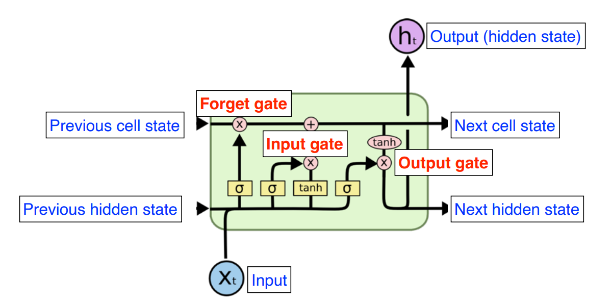
Xt : t번째 input (ex)단어
ht : t번째 state의 Output -> 여기서는 hidden state라 칭함
Previous cell state : 0~t까지의 정보를 Summary해준 정보(내부에서만 흘러감) => 이게 핵심임
Previous hidden state(=Previous output) : 위로도 흘러가고 직진도 함 (t+1번째 LSTM에 Previous hidden state로 들어감)
Output : 다음번 단어의 확률을 찾겠다(Output 말고도 다음 hidden state로 보내준다)

그래서 LSTM의 입력으로 들어오는 것은

t번째 의 Input
이전의 출력인 Previous hidden state
그리고 밖으로 나가지 않고 지금까지의 과거를 요약한 Previous cell state 이다

즉, cell 단위로 봤을 때 들어오는 거 3개 나가는 거 3개지만 실제로 나가는 것은 1개이다

어떻게 RNN의 문제점인 short term dependency를 해결할 수 있었을까?

Cell state가 지금까지의 정보를 요약하고 내부에서만 흘러간다. (이게 핵심 정리라고 생각하면 된다)

왜 핵심정리라고 했나면

Forget gate를 통해서 중요한 정보만을 선별한다

Update gate에서 Forget gate에서 넘어온 정보와 현재 정보를 적절히 섞어서 갱신(이전거에서 버릴 건 버리고 들어온 것 중 일부를 갱신)

Output gate에서 어떤 걸 밖으로 뽑아 낼지 한번 더 결정

이렇게 하면 무지성으로 교과서를 암기하는 것이 아닌 핵심만 정리해서 머리속에 넣는 느낌을 줄 수 있다

여기서 더 심화하면 GRU(Gate Recurrent Unit)이 있긴 하다 : Reset Gate랑 Update Gate만으로 모델 구성

LSTM -> GRU

어쩌피 hidden 계속 넘어가는데 이걸 이용해서 ouput 만들면 되지 않냐

LSTM보다 성능이 더 좋을 때가 많음

(Parameter는 적은데 성능이 비슷 = 일반화를 더 잘한다)

Sequential data를 해결하기 위해 RNN이 나왔고
RNN이 가진 단점(long-term dependencies를 못 잡음)을 해결하기 위해 LSTM이 등장하였고
LSTM의 Parameter를 줄이기 위해 Output Gate를 빼고 Reset gate와 Update gate를 둔 GRU가 나오고
GRU의 성능이 parameter가 적음에도 좋은 성능을 보인다

Transformer의 등장

위에 모델들을 보면 너무 Recursive에 한정되어있는 것을 볼 수있다

그게 왜?

병렬처리가 불가능하다는 큰 단점이 있다(이 전 결과에 의존하게 되어서)

Transformer는 Recursive 구조를 과감히 없애고 attention 구조를 제시한다.

예전에 Diffusion을 다루면서 한번 간략하게 소개한 적이 있지만 https://aisj.tistory.com/199

이번엔 논문 구현과 Pytorch 기본적인 사용

그리고 Sequential Data에 대한 Transformer 를 적용하는 방법

논문 리뷰등을 위주로 다룰 예정이다

논문 링크

https://arxiv.org/abs/1706.03762

Attention Is All You Need

The dominant sequence transduction models are based on complex recurrent or convolutional neural networks in an encoder-decoder configuration. The best performing models also connect the encoder and decoder through an attention mechanism. We propose a new

arxiv.org

Attention Is All You Need (2017)

제일 먼저 제목에서 이 논문을 함축한 것을 볼 수 있다.

너가 찾고자 하는 것 너가 필요로 하는 것은 Attention에 전부 있다는 뜻이다

여기서 짚고 넘어갈 것은 대체 왜 sequence Data 처리가 어렵다고 하는 것일까 이다

우리의 일상생활을 생각해보자

표준 문장을 적어보면 "승종아, 오늘 점심에 밥 먹었어?"

이런 문장이

"승종, 밥 먹었어?" , "승종, 점심에 밥 먹었어?" , "승종, 점심 먹었어?" 등등 길이가 달라지고 어순이 달라지고 등등

하나의 동일한 의미에 다양한 문장을 만들 수 있다

즉 Original sequence에 대해서

Trimmed Sequence(마지막 몇개의 단어의 생략)
Omitted Sequence (중간에 몇개의 단어의 생략)
Permuted Sequence (어순이 달라지는 경우)

등 많은 변화가 있을 수 있다

이런 변화에 적응하여 단순히 위에 같이 Hidden cell을 추가해 요약하면서 가겠다해도

전체 문장을 고려한 문맥을 파악하기는 어렵다

이러한 Task에 대한 해결점으로

Transformer는 기본적으로 Self attention이라는 구조를 사용한단

Keypoint는 다음과 같다

1. N개의 단어가 어떻게 한번에 처리가 되는지
2. Encoder와 Decoder 사이에 어떤 정보를 주고 받는지
3. Decoder가 어떻게 Generation 할 수 있는지

Abstract

The dominant sequence transduction models are based on complex recurrent or convolutional neural networks that include an encoder and a decoder.

현재(2023년) 기준으로는 Sequential 모델? 자연어 번역? 그건 Transformer이용해야지 라고 말하지만

이때는 Encoder 와 Decoder로 구성한 CNN ex) VAE(Auto Encoding Variational Bayes) https://arxiv.org/abs/1312.6114

혹은 Recurrent structure(위에서 설명한 RNN, LSTM 같은 것들)로만 구현하던 시대이다.

We propose a new simple network architecture, the Transformer, based solely on attention mechanisms, dispensing with recurrence and convolutions entirely.

이에 대해 새로운 구조를 Transformer 제시한다고 한다.

We show that the Transformer generalizes well to other tasks by applying it successfully to English constituency parsing both with large and limited training data.

한정된 데이터에서 영어 구문 분석 같은 것에서 두각을 보인다고 한다.

## Make Data 구현

자 그러면 Sequential Data를 만들어 보자

물론 이중 list 선언하고 for문을 돌려서 Sequential Data를 만들 수 있다

import random as rd
import numpy as np
raw_data = []
col = 80
row = 20
for c in range(col):
    raw_data.append([rd.randint(0,100) for _ in range(row)])
raw_data = np.array(raw_data)
print(raw_data)
print(raw_data.shape)

하지만 본인은 주식 데이터가 있어서 이를 이용하였다 (csv 파일)

import pandas as pd
raw_data = pd.read_csv('./data/raw_data.csv', parse_dates=['trd_dt'])
#parse_dates는 날짜 처럼 사용하기 위해

이렇게 하면 사실 항목이 엄청 많아서 이 중 어떤 것을 뽑을지 고민할 수 있다.

주식이면 시가, 종가, 거레대금 등등....

본인은 제일 많이 사용하는 피어슨 상관계수를 이용하였다

import seaborn as sns
corr = (raw_data.corr(method = 'pearson'))


#가시화 부분
raw_col = [c for c in raw_data.columns]
sns.set(font_scale = 0.7)
hm = sns.heatmap(corr.values,
                 cbar = True,
                 annot = True,
                 square = True,
                 fmt = '2f',
                 annot_kws = {'size' : 4},
                 xticklabels = raw_col,
                 yticklabels = raw_col
                )

1. Information

Recurrent neural networks, long short-term memory [13] and gated recurrent [7] neural networks in particular, have been firmly established as state of the art approaches in sequence modeling and transduction problems such as language modeling and machine translation
.......

In this work we propose the Transformer, a model architecture eschewing recurrence and instead relying entirely on an attention mechanism to draw global dependencies between input and output.

위에서 번역한 Abstract를 반복한 말이다.

핵심은 Draw dependencies between input and output이라고 생각을 하는데

input과 output 전체의 문맥의 의존성을 파악하는 방법이라 설명하고 있다

2. Background

...... the number of operations required to relate signals from two arbitrary input or output positions grows in the distance between positions, linearly for ConvS2S and logarithmically for ByteNet.This makes it more difficult to learn dependencies between distant positions.

기존에 있던 ConvS2S나 ByteNet 같은거의 문제점은 "그녀가 뛴다."라는 문장을 번역할 때는 문제가 되지 않지만

"그녀가 내가 나왔던 학교 옆에 있는 중학교에 농구장을 내 친구랑 함께 어제 밥도 먹지 않고 뛰었다" 이런 문장에 있어서는 문맥파악이 어렵다는 것이다

Self-attention, sometimes called intra-attention is an attention mechanism relating different positions of a single sequence in order to compute a representation of the sequence.

이런 어려움을 문장의 표현을 계산하기 위해 단일 sequence의 서로다른 위치와 관련된 정보를 뽑아내는 알고리즘이라고 한다.

## Data / Dataloader 구현

밑에 모델을 만들고 돌리기 위해서는 Data와 Dataloader를 구현해야 한다.

우리는 지금 Sequence Data를 다루고 있는데 내가 만든 데이터는 1043행을 총 4937개를 가지고 있는 DataFrame이다

이걸 그대로 Transformer에 가져다 넣으면 OOM이 발생한다.

이를 위해 Batch training방법을 사용해야 하고 자연스럽게 torch.utils.data에 있는 DataLoader와 Dataset을 사용하였다.

딥러닝에서 배치는 모델의 가중치를 한번 업데이트시킬 때 사용되는 샘플들의 묶음을 의미합니다
즉, 1000개의 데이터에 batch size가 20이라면 20개의 데이터를 학습하고 가중치를 업데이트하고 하는 작업을 50번 반복한다.
이때 배치사이즈가 너무 크면 학습속도도 느려지고 Memory문제가 발생한다. 하지만 너무작은 batch를 사용해도 샘플을 50개를 학습하고 업데이트할 때보다 1개 학습하고 업데이트 하는 방법은 보기에도 학습이 불안정하게 만들 수 있다는 뜻이다. (이때 batch size=1이면 SGD(Stochastics Gradient Descent 방법이라고 한다)

Gradient Descemt
- 현제 네트워크에 내가 가진 데이터셋 전체의 에러를 구하고 기울기를 계산해서 업데이트하는 방법
- 장점
  - 전체 데이터에 대해 한번에 처리하여서 업데이트 횟수가 적고 학습이 비교적 안정적이다
  - 꽤나 정확한 최적값을 찾아 갈 수 있다 하다
- 단점
  - 한 step 가는데 너무 오래 걸린다
  - 제일 중요한 건 local minimum에 한번 빠지면 답이 없다
  - 그리고 엄청 큰 메모리가 필요하다(위에서 말한 것과 동일)
Stochastic Gradient Descent
- 쉽게 배치 사이즈가 1로 데이터 하나보고 업데이트하고 하나보고 업데이트 하는 방식이다
  - 문제하나 풀고 답보고 하나풀고 답보고
- 근데 왜 확률적(Stochastic)이라는 말이 붙었을까
  - 데이터 세트에서 무작위로 균일하게 선택한 하나의 데이터를 사용하기 때문에
- 장점
  - 빠르다
- 단점
  - 수렴속도가 느리다
  - 놀고있는 GPU용량을 보면 화가난다
  - 너무 튀어서 Global minimum을 찾지 못활 수도 있다
Mini Batch Gradient Descent (MSGD)
- 위에 SGD를 저렇게 하지 말고 일정한 size마다 샘플링을 해서 GD처럼 계산하면 되지 않냐라는 아이디어
- 장점
  - GD보다는 local minimum 에 빠질 가능성 적음
  - SGD 보다는 Global minimum찾을 확률 있음
  - 좀 애매한 포지션 (GD 와 SGD 합친 느낌)인데 또 성능은 괜찮아
- 단점
  - batch size라는 hyperparameter 찾기 귀찮음

Batch 경사 하강법 1회에 사용되는 데이터의 묶음을 의미
Batch Size = 전체 학습 데이터: 배치 경사 하강법(BGD)
Batch Size = 1: 확률적 경사 하강법(SGD)
Batch Size = batch_size(사용자 지정)

자세한건 이거 보면 좋을 것 같다 https://sjpyo.tistory.com/56

이정도만 하고 본론으로

다음과 같이 코드를 사용하였다

from torch.utils.data import DataLoader,Dataset,random_split
device = "cuda" if torch.cuda.is_available() else "cpu"
class CustomDataset(Dataset):
    def __init__(self,x_data,y_data,device):
        x_data = x_data.to_numpy() #DataFrame to numpy
        y_data = y_data.to_numpy() #DataFrame to numpy
        self.data = torch.LongTensor(x_data).to(device)
        # self.data = torch.FloatTensor(x_data).to(device)
        self.label = torch.LongTensor(y_data).to(device)
        # self.label = torch.FloatTensor(y_data).to(device)

    def __len__(self):
        return len(self.x_data)

    def __getitem__(self, idx):
        # x = torch.FloatTensor(self.data[idx]).to(device)
        # y = torch.FloatTensor(self.label[idx]).to(device)
        # #self.x_data와 self.y_data가 이미 GPU(CUDA)로 이동되어 있기 때문에, __getitem__ 메서드에서 다시 .to(device)를 사용하지 않아야 합니다. 

        x = self.data[idx]
        y = self.label[idx]

        return x, y


dataset = CustomDataset(x_train,y_train,device)


dataset_size = len(dataset)
train_size = int(dataset_size * 0.8)
validation_size = dataset_size - train_size

train_dataset, validation_dataset = random_split(dataset, [train_size, validation_size])
test_dataset = CustomDataset(x_test,y_test,device)

print(f"Training Data Size : {len(train_dataset)}")
print(f"Validation Data Size : {len(validation_dataset)}")
print(f"Testing Data Size : {len(test_dataset)}")

train_dataloader = DataLoader(
    train_dataset, 
    batch_size=16, 
    shuffle=False, 
    drop_last=True)

validation_dataloader = DataLoader(
    validation_dataset, 
    batch_size=4, 
    shuffle=False, 
    drop_last=True)

test_dataloader = DataLoader(
    test_dataset, 
    batch_size=1, 
    shuffle=False, #순서대로 이용하기 위해서 
    drop_last=False)

이렇게 하면 데이터 세팅이 완료된다

3. Model Architecture

the encoder maps an input sequence of symbol representations (x1, ..., xn) to a sequence of continuous representations z = (z1, ..., zn). Given z, the decoder then generates an output sequence (y1, ..., ym) of symbols one element at a time

제일 간단하게 다음과 같이 구조를 나타낼 수 있다

input X= (x1, ..., xn) -> [Encoder] -> continuous representation Z=(z1, ..., zn) -> [Decoder] -> Output Y = (y1, ..., ym)

여기서 주의점은 다음과 같다고 생각한다

1. input size = n , output size = m // 즉 입력과 출력의 크기가 달라도 상관이 없다는 뜻이다.

2. Encoder-Decoder구조는 이미 나와있는 상태였다 (이게 트렌스포머 논문에서 나왔다 하면 바보야)

.At each step the model is auto-regressive [10], consuming the previously generated symbols as additional input when generating the next

생성할 때 이전 생성된 기호를 추가적인 입력으로 사용한다고 한다(Decoder단에 관한 설명인거 같다)

사실 위에 사진보다

이게 더 좋은 그림같다.

The Transformer follows this overall architecture using stacked self-attention and point-wise

self attention이랑 point-wise 쌓아서 만든다고 한다.

3.1 Encoder and Decoder Stacks

Encoder

The encoder is composed of a stack of N = 6 identical layers

얘네는 Encoder 6개 쌓아서 만들었다고 한다

Each layer has two sub-layers. The first is a multi-head self-attention mechanism, and the second is a simple, positionwise fully connected feed-forward network.

Encoder 자세히 보면 주황색하고 파란색 sub-layers가 있는 것이 보일 것이다

이렇게 두개의 Sublayer로 구성한다

Multi-head self-attention
position-wise fully connected feed-forward network

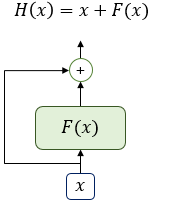
. We employ a residual connection [11] around each of the two sub-layers, followed by layer normalization

residual connection : 머리를 꼬리에 붙이는 것 (Output을 그대로 input으로 넣음)

That is, the output of each sub-layer is LayerNorm(x + Sublayer(x)), where Sublayer(x) is the function implemented by the sub-layer itself

그렇기 때문에 Encoder output = LayerNorm(x + Sublayer(x)) 이런식의 결과가 나오는 것이다

To facilitate these residual connections, all sub-layers in the model, as well as the embedding layers, produce outputs of dimension d_model = 512.

자 Encoder에서 나온 출력을 그대로 Encoder로 넣는다고 했다

그러면 Encoder의 입력 layer와 출력 layer의 dimension이 동일해야하는 것은 자명하다 (d_model 이라는 값으로 동일하다고 가정)

Encoder 6개를 다음과 같이 E1,E2 ..... E6로 나타낼 때

1. E1은 Embedding layer를 지난 결과 값을 받는다 -> E1의 input dimension은 d_model이다 -> Embedding layer의 output도 d_model이여야 한다

2. E6은 Encoder의 최종 출력으로 그대로 모델에 들어가게 된다 -> E6의 output과 모델의 input dimension이 같아야한다 -> E6의 dimension은 d_model 이다 -> 모델의 input도 d_model 이다

즉 다음은 모두 같은 값이다

Embedding output dimension

= Encoder input dimension

= Encoder output dimension

= Model input dimension(Model dimension)

아래 예시에서도 확인할 수 있다

https://welcome-to-dewy-world.tistory.com/108

이렇게 보면 하나의 Decoder에 Encoder 결과가 넘어가는 것처럼 보이지만

엄밀하게는 다음 그림과 같다

그러면 결국 Encoder 6에 의존되는 거 아니냐는 말에는

위에서 설명한 Residual connection 때문에

이런 식의 그림이 나온다

즉,

와 같이 input을 그대로 output과 합쳐주어

이렇게 다음 Encoder로 넘겨준다

그래서 Add 라는 말이 있는 것이고

Norm은 Normalization으로

위 과정을 통해 나온 output을 정규화 시킨다.

각각의 token에 대해 다른 파라미터를 주어

이렇게 정규화를 하고

분모의 입실론은 분모가 0이 되는 것을 막는 용도이다

이렇게 나온 결과를 r,B 감마 베타를 이용하여 (학습 가능)

초기를 다음과 같이 세팅하고

아래의 식으로 정규화 결과를 구현한다

thinking : (4,2,3,5), machines : (2,1,-3,2)의 Vector로 표현된다고 가정하자

thinking의 평균은 3.5, 1.11이고 machines의 평균은 0.5, 표준편차는 2.06이다.
이를 활용하여 Batch Normalization을 수행하면,
thinking : (0.65, -0.45, -1.35, 1.25),
machines : (0.7, -1.5, -0.3, 1.1)의 Vector로 변환되게 된다.

이후 Affine Transformation을 수행해준다.
Layer의 Node별로 수행해줘야 하기 때문에,
총 4개의 함수가 필요할 것이다 (단어 Vector의 Dimension마다 적용시킬 함수가 존재해야 함)
Dimension = 1에는 y = 3x + 1,
2일 떄는 y = x+1,
3일 때는 y = -x,
4일 때는 y = -2x+2를 적용시킨다고 가정하자.
그렇다면, Layer Normalization을 거친 최종 Vector 값은
Thinking : (2.95, 0.55, 1.35, -0.5),
Machines : (3.1, -0.5, 0.3, -0.2)가 될 것이다.

https://velog.io/@idj7183/Attention-TransformerSelf-Attention

Decoder

The decoder is also composed of a stack of N = 6 identical layers.

decoder도 6개 쌓아 올렸다고 한다

the decoder inserts a third sub-layer, which performs multi-head attention over the output of the encoder stack

Encoder 는 다음과 같은 sub-layer를 가지고

Multi-head self-attention
position-wise fully connected feed-forward network

Decoder는 여기에 하나 추가한

Multi-head self-attention (위에 그림에서는 Masked Multi head Attention이라 명시)
Multi-head self-attention (with output of Encoder)
position-wise fully connected feed-forward network

Similar to the encoder, we employ residual connections around each of the sub-layers, followed by layer normalization

얘도 D1에서 D2로 출력이 Normalization거친 다음 그대로 입력으로 들어가는 구조라 한다.

We also modify the self-attention sub-layer in the decoder stack to prevent positions from attending to subsequent positions.

Self attention 구조가 Encoder랑은 조금 다르게 가공했다고 한다

(약간의 의역을 하자면 다음 순서에 있는게 뭔지 보지 못하도록 수정했다는 말 같다 : Masking)

This masking, combined with fact that the output embeddings are offset by one position, ensures that the predictions for position i can depend only on the known outputs at positions less than i.

이 문장은 두 문장으로 쪼개서 해석하는 것이 좋을 것 같다

This masking, combined with fact that the output embeddings are offset by one position

(별로 중요한 문장 아닌 듯) 마스킹은 하나의 position에서 offset 되어 output embeddings이 만들어진다는 사실을 결합하여

(한 위치에 필요한 단어가 하나씩 나온다 이런 뜻? 약간 I 다음에는 동사가 오고 동사가 다음에는 목적어가 온다 이런느낌)

ensures that the predictions for position i can depend only on the known outputs at positions less than i.

위에 방법은 i위치에서의 예측은 i미만의 위치에서만 의거하여 예측할 수 있도록(뒤쪽을 보지 못하도록) 해준다.

## Target mask 구현

    def get_tgt_mask(self, size) -> torch.tensor:
    	'''
        tensor([[0., -inf, -inf, -inf],
                [0., 0., -inf, -inf],
                [0., 0., 0., -inf],
                [0., 0., 0., 0.]]) 를 만들어주는 작업 (size는 입력받는다 (정사각형 행렬)예시는 4)
        '''
        mask = torch.tril(torch.ones(size, size) == 1) # Lower triangular matrix(하삼각함수)
        mask = mask.float()
        mask = mask.masked_fill(mask == 0, float('-inf')) # Convert zeros to -inf
        mask = mask.masked_fill(mask == 1, float(0.0)) # Convert ones to 0
 
        return mask

3.2 Attention

An attention function can be described as mapping a query and a set of key-value pairs to an output, where the query, keys, values, and output are all vectors.

Attention이란 Query와 key values 쌍을 (Query 랑 key,value를 구분한 이유는 이따가 나옴) output 과 mapping시키는 것이다

output과 query, keys, values, output은 vectors라고 한다

-> Decoder에서 출력 단어를 예측하는 시점마다 Encoder에서의 전체 입력 문장을 다시 한번 참고하는 것 (연관있는 단어에 좀더 집중(Attention 하겠다))

여기서 부터 여럽다고 느낄 수 있는데 생각보다 단순하다

다음 블로그를 참고하자

http://jalammar.github.io/illustrated-transformer/

The Illustrated Transformer

Discussions: Hacker News (65 points, 4 comments), Reddit r/MachineLearning (29 points, 3 comments) Translations: Arabic, Chinese (Simplified) 1, Chinese (Simplified) 2, French 1, French 2, Italian, Japanese, Korean, Persian, Russian, Spanish 1, Spanish 2,

jalammar.github.io

"Thinking Machines"라는 단어가 들어오면 Embedding layer를 통해 다음과 같은 Embedding vector (X1 , X2)가 나온다

이 X1, X2 에 WQ, WK, WV를 곱해서 각각의 Queried, Keys, Values Vector를 만든다

The output is computed as a weighted sum of the values, where the weight assigned to each value is computed by a compatibility function of the query with the corresponding key.

Output은 weighted sum of the values라고 한다,

그러면 우리가 output을 구하기 위해서는 다음을 계산해야 한다.

Weight
values (이건 이미 구함)

이제 Weight를 어떻게 만드냐가 관건인데 이건 뒤에서 softmax의 결과이다(3.2.1에 나옴)

논문에서는 이를 Query 와 이에 상응하는 Key의 compatibility function(적합성/호환성 함수)에 의해 weight가 계산된다고 한다

-> 이를 의역하자면 어떤 value가 연관성이 높을까를 Query와 key을 어떻게 뽀짝뽀짝해서 만든다는 뜻이다 (이 방법이 Scaled Dot Product Attention)

3.2.1 Scaled Dot-Product Attention

We call our particular attention "Scaled Dot-Product Attention"

논문 읽기 전에는 transformer 는 self attention 이용해서 ~ 라고 말하는데 Scaled Dot-product attention이라고 엄밀히 정의 해주고 있다

The input consists of queries and keys of dimension dk, and values of dimension dv

위에 보면 dk, dv가 만들어 진것을 볼 수 있다

더 정확한 이해를 위해서 Wk의 shape를 적어보면 다음과 같다 (d_embedding, dk) -> 이러면 결과가 dk지

We compute the dot products of the query with all keys, divide each by √ dk, and apply a softmax function to obtain the weights on the values.

이 문장을 두 문장으로 나눠보자

We compute the dot products of the query with all keys

Score 를 구하는 방법을 알려주고 있다.

Thinking의 query인 q1을 Thinking, Machines 모두의 key와 dot product를 진행한다.

즉, 구하고자 하는 단어의 Queries에 대해 모든 단어의 (자기자신 포함) Keys 값을 내적한다

ex) q1 dot k1 = (10,1,3)(10,6,4) = 112

이는 내가 encoding 하고자 하는 단어의 Queries 벡터와 나머지 모든 N에 대한 keys vector를 내적하여 각각 단어끼리의

유사도를 파악 한다 -> 이것이 Attention (특정 time step에 어떤 입력을 주의 깊게 볼지 결정)

쉽게 유사도를 key랑 queries 내적으로 구하겠다는 말이다

divide each by √ dk, and apply a softmax function to obtain the weights on the values.

여기에 √ dk 를 나누어 준다 (Scaling) 이는 softmax때문에 사용한다

softmax는 입력받은 값을 출력으로 0~1사이의 값으로 모두 정규화하며 출력 값들의 총합이 항상 1이 되게 해준다.

구현은 이렇게 할 수 있다

import numpy as np

def softmax(x):
    e_x = np.exp(x - np.max(x))
    return e_x / e_x.sum()

나누어 주는 이유는 매우 간단한데 dot product 결과가 [1,200] 의 shape를 가지고 각각 값들이 100 이상이라고 해보자

만약 q1 k1 = 112이라고 했을 때 softmax를 하면 최대값은 112/ 100*200이 되고 거의 0이다.

뿐만아니라 대부분의 값들 모두 0과 비슷하게 나오는 현상이 발생하기 때문에 이를 방지하고자 한 행위이다.

보면 이 softmax 결과가 the weights on the values 라고 한다.

위에서 우리가 구해야하는 두가지가

Weight
values (이건 이미 구함)

라고 했는데 Weight를 구했네?

그럼 이걸 곱하는 weighted sum of the values를 해주면 Output이 나온다

(위에서 구한 Attention Weight는 스칼라 값이므로 여기에 각각의 단어의 Value를 곱해서 더해주면 최종 출력이 나온다)

이러한 과정을 거치기 떄문에 최종 출력인 Encoding Vector는 Value vector와 동일한 차원을 가지게 된다

이를 수식으로 표현하면 다음과 같다

즉, Value Vector들의 weight를 구하는 방법이 ~ softmax까지 하여서 Attention Weight를 구하는 것이고

최종적으로 나오는 encoding vector는 value vector와 weighted Sum을 진행한 값이다

그리고 그림으로 표현하면

로 나타낼 수 있다

못보던 Mask가 왜 갑자기 옵션으로 붙었냐

Decoder에서 Masked Multi-Head Attention을 사용할 때 이용하기 위해서 달아주었다

(순차적으로 데이터를 만들어 내기 원하고 순서가 되지 않은 정보는 Attention 시키지 않게 하기 위해서)

그래서 구현도 get_tgt_mask() 가져다가 쓰면 된다.

요약
Query : 연관성을 찾고자 하는 단어 (하나여서 이것만 단수로 쓰는 것을 볼 수 있음)
Keys: 연관성이 있을 법한 단어들
Values : 얼마나 영향력이 있는지

.... Dot-product attention is identical to our algorithm, , except for the scaling factor of 1 / √ dk .

scaling을 뺀 Dot-product는 얘네가 상용한 거랑 매우 흡사하다고 한다

그럼 자기네들은 뭐가 다르냐

Additive attention computes the compatibility function using a feed-forward network with a single hidden layer.

Feed Forward 붙인게 다르다고 한다 (허허..)

위에 과정을 요약해보면 다음과 같다

The first step is to calculate the Query, Key, and Value matrices. We do that by packing our embeddings into a matrix X, and multiplying it by the weight matrices we’ve trained (WQ, WK, WV).

위의 그림에서 X는 앞에서 예시를 들었던 "Thinking Machines"를 Matrix로 embedding 한 것이다

가로는 Embedding 할 때 정의하는 demension이고

세로는 단어의 개수 즉, 2 이다

그림과 같은 방법으로 Q K V를 구하고

다음 연산을 진행하면 z가 나오게 된다

굉장히 복잡해보이지만 Python을 통해 한 줄로 구현이 가능한 수식이다

Scores = Q.matmul(K.transpose(-2,-1)) / np.sqrt(d_K)

위에서 볼 수 있듯이 각각 단어들에 대해서 동일한 WQ, WK, WV를 통해서 Q,K,V를 만들어 낸다

지금 머리 속에 생각한 걱정

이러면 조금 성급한 일반화가 되지 않을까? 성능이 좋게 나올까? 라는 생각을 나도 했는데

조금 더 읽고 나서 이러한 걱정이 해결되었다

3.2.2 Multi-Head Attention

이게 논문의 그림이긴 한데 제일 Best는 이 그림이다

논문 읽어나가기 전에 직관적으로 이해하면

위에 그림은 number of heads가 8인 그림이다

위에서 진행한 single head attention과정을 8번 반복하여 output인 Z0,Z1,.....Z7을 만들고

이를 단순하게 concat 시킨다

위 그림 기준으로는 [3*8,2] shape를 가지는 matric 이 만들어진다.

이걸 Linear layer 하나를 통과 시켜서 최종 결과를 만들어 내는 방법이다

Instead of performing a single attention function with dmodel-dimensional keys, values and queries, we found it beneficial to linearly project the queries, keys and values h times with different, learned linear projections to dk,
dk and dv dimensions, respectively.

아싸리 Single head로 keys, values, queries의 dimension을 모델의 차원과 동일하게 가져가는 것이 아닌

key,value, query들에 각각 다르게 학습된 lineart projection을 h개의 (h번의) attention을 진행하는 것이 좋은 것을 발견 했다고 한다.

이걸 수식으로 나타내면 다음과 같다

논문에서는 hyperparameter를

d_model = 512

dk=dv = 64 (= d_model/num_head)

num_head = 8로 진행했다고 한다(single일때랑 계산복잡도 유사하게 하고 싶어서)

single head일때는

dk=dv =d_model = 512로 진행했거든...

(추가로 key, value의 차원은 동일할 필요없다 / 단 Query 와 key의 차원은 동일해야한다(내적 때문에))

이제 구현해보자

## Transformer 구현

import math
import torch
import torch.nn as nn
import torch.nn.functional as F
import torch.optim as optim

class Transformer(nn.Module):
    # Constructor
    # 기존에는 in_num_tokens와 oout_num_tokens를 동일하게 num_tokens로 받았습니다.
    def __init__(self,in_num_tokens, out_num_tokens, dim_model, num_heads, num_encoder_layers, num_decoder_layers, dropout,device):
        super().__init__()
        
        
        self.dim_model = dim_model
        self.device = device


        # x_val , x_train -> numpy.ndarray
        # LAYERS를 샇아줍니다
        # 위에서 정의한 positionalEncoding을 사용합니다.
        self.positional_encoder = PositionalEncoding(
            dim_model=dim_tunning,
            dropout=0.1, 
            max_len=3000)



        # Embedding을 해줍니다
        self.embedding = nn.Embedding(
            num_embeddings=in_num_tokens, #임베딩할 단어들 개수
            embedding_dim=dim_model, #임베딩할 벡터의 차원
            device=device)

        self.transformer = nn.Transformer(
            d_model=dim_model,
            nhead=num_heads,
            num_encoder_layers=num_encoder_layers,
            num_decoder_layers=num_decoder_layers,
            dim_feedforward = 128,
            dropout=dropout,
            device=device
        )

        #nn.Transformer(d_model=1040,nhead=4, num_encoder_layers=3, num_decoder_layers =3,dim_feedforward =128,device=device)
        #in_features, out_features, bias=True, device=None,  -> expected : dim_model , 5. , cuda
        self.out = nn.Linear( #마지막 단에 나오는 LAYER
            dim_model,
            out_num_tokens,
            device=device)
 
    def forward(self, src, tgt, tgt_mask=None, src_pad_mask=None, tgt_pad_mask=None):
        # src, Tgt size -> (batch_size, src sequence length)
        # [seq_len, batch_len, embedding_dim]
        
        # Embedding + positional encoding - Out size = (batch_size, sequence length, dim_model)
        #print("start for embedding and positional_encoder for",self.device)
        src = self.embedding(src) * math.sqrt(self.dim_model)
        tgt = self.embedding(tgt) * math.sqrt(self.dim_model)
        src = self.positional_encoder(src)
        tgt = self.positional_encoder(tgt)

        #print("positional_encoder for ",self.device," complete")
        # Transformer blocks - Out size = (sequence length, batch_size, num_tokens)
        # print(src.shape)
        # print(tgt.shape)
        transformer_out = self.transformer(src, tgt, tgt_mask=tgt_mask, src_key_padding_mask=src_pad_mask, tgt_key_padding_mask=tgt_pad_mask)
        out = self.out(transformer_out) #linear layer단을 지납니다
        return out

    
    def get_tgt_mask(self, size) -> torch.tensor:
        '''
        tensor([[0., -inf, -inf, -inf],
                [0., 0., -inf, -inf],
                [0., 0., 0., -inf],
                [0., 0., 0., 0.]]) 를 만들어주는 작업 (size는 입력받는다 (정사각형 행렬))
        '''
        #batch_size == 8
        mask = torch.tril(torch.ones(size, size) == 1) # Lower triangular matrix(하삼각함수)
        mask = mask.float()
        mask = mask.masked_fill(mask == 0, float('-inf')) # Convert zeros to -inf
        mask = mask.masked_fill(mask == 1, float(0.0)) # Convert ones to 0
 
        return mask
 
    def create_pad_mask(self, matrix: torch.tensor, pad_token: int) -> torch.tensor:
        #padding token = -(1e+5) 
        return (matrix == pad_token)

와 같이 구현을 할 수 있는데 나는 조금 더 커스텀해서

다음 그림처럼

import math
import torch
import torch.nn as nn
import torch.nn.functional as F
import torch.optim as optim

class Transformer(nn.Module):
    # Constructor
    # 기존에는 in_num_tokens와 oout_num_tokens를 동일하게 num_tokens로 받았습니다.
    def __init__(self,dim_tunning,dim_tunned,in_num_tokens, out_num_tokens, dim_model, num_heads, num_encoder_layers, num_decoder_layers, dropout,device):
        super().__init__()
        
        
        self.dim_model = dim_model
        self.device = device


        # x_val , x_train -> numpy.ndarray
        # LAYERS를 샇아줍니다
        # 위에서 정의한 positionalEncoding을 사용합니다.
        self.positional_encoder = PositionalEncoding(
            dim_model=dim_tunning,
            dropout=0.1, 
            max_len=3000)



        # Embedding을 해줍니다
        self.embedding = nn.Embedding(
            num_embeddings=in_num_tokens, #임베딩할 단어들 개수
            embedding_dim=dim_tunning, #임베딩할 벡터의 차원
            device=device)
        
        self.tunning1 = nn.Linear( #embedding 다음 붙는 LAYER
            dim_tunning,
            dim_tunned,
            device=device)
        
        self.fc = nn.Linear( #embedding 다음 붙는 LAYER
            dim_tunned,
            dim_tunned,
            device=device)

        self.tunning2 = nn.Linear( #embedding 다음 붙는 LAYER
            dim_tunned,
            dim_model,
            device=device)

        self.transformer = nn.Transformer(
            d_model=dim_model,
            nhead=num_heads,
            num_encoder_layers=num_encoder_layers,
            num_decoder_layers=num_decoder_layers,
            dim_feedforward = 128,
            dropout=dropout,
            device=device
        )

        #nn.Transformer(d_model=1040,nhead=4, num_encoder_layers=3, num_decoder_layers =3,dim_feedforward =128,device=device)
        #in_features, out_features, bias=True, device=None,  -> expected : dim_model , 5. , cuda
        self.out = nn.Linear( #마지막 단에 나오는 LAYER
            dim_model,
            out_num_tokens,
            device=device)
 
    def forward(self, src, tgt, tgt_mask=None, src_pad_mask=None, tgt_pad_mask=None):
        # src, Tgt size -> (batch_size, src sequence length)
        # [seq_len, batch_len, embedding_dim]
        
        # Embedding + positional encoding - Out size = (batch_size, sequence length, dim_model)
        #print("start for embedding and positional_encoder for",self.device)
        src = self.embedding(src) * math.sqrt(self.dim_model)
        tgt = self.embedding(tgt) * math.sqrt(self.dim_model)
        src = self.positional_encoder(src)
        tgt = self.positional_encoder(tgt)

        tun = self.tunning1(src)
        tun = self.fc(tun)
        src = self.tunning2(tun)
        
        tun = self.tunning1(tgt)
        tun = self.fc(tun)
        tgt = self.tunning2(tun)


        #print("positional_encoder for ",self.device," complete")
        # Transformer blocks - Out size = (sequence length, batch_size, num_tokens)
        # print(src.shape)
        # print(tgt.shape)
        transformer_out = self.transformer(src, tgt, tgt_mask=tgt_mask, src_key_padding_mask=src_pad_mask, tgt_key_padding_mask=tgt_pad_mask)
        out = self.out(transformer_out) #linear layer단을 지납니다
        return out

    
    def get_tgt_mask(self, size) -> torch.tensor:
        '''
        tensor([[0., -inf, -inf, -inf],
                [0., 0., -inf, -inf],
                [0., 0., 0., -inf],
                [0., 0., 0., 0.]]) 를 만들어주는 작업 (size는 입력받는다 (정사각형 행렬))
        '''
        #batch_size == 8
        mask = torch.tril(torch.ones(size, size) == 1) # Lower triangular matrix(하삼각함수)
        mask = mask.float()
        mask = mask.masked_fill(mask == 0, float('-inf')) # Convert zeros to -inf
        mask = mask.masked_fill(mask == 1, float(0.0)) # Convert ones to 0
 
        return mask
 
    def create_pad_mask(self, matrix: torch.tensor, pad_token: int) -> torch.tensor:
        #padding token = -(1e+5) 
        return (matrix == pad_token)

로 구현했습니다.

3.2.3 Applications of Attention in our Model

The Transformer uses multi-head attention in three different ways:
• In "encoder-decoder attention" layers, the queries come from the previous decoder layer, and the memory keys and values come from the output of the encoder. This allows every position in the decoder to attend over all positions in the input sequence. This mimics the typical encoder-decoder attention mechanisms in sequence-to-sequence models such as [38, 2, 9].
• The encoder contains self-attention layers. In a self-attention layer all of the keys, values and queries come from the same place, in this case, the output of the previous layer in the encoder. Each position in the encoder can attend to all positions in the previous layer of the encoder.
• Similarly, self-attention layers in the decoder allow each position in the decoder to attend to all positions in the decoder up to and including that position. We need to prevent leftward information flow in the decoder to preserve the auto-regressive property. We implement this inside of scaled dot-product attention by masking out (setting to −∞) all

3가지 다른 방법으로 multi-head attention을 사용한다고 한다.

encoder-decoder attention layers
- Query : 이전의 Decoder layer에서 넘어온다
- Key, Values : Encoder layer의 output에서 넘어 온다.
- 이것은 모든 decoder에서 만들어지는 값은 input sequence의 모든 단어를 참고해서 만들 수 있게 해준다
- 전통적인 encoder-decoder attention 메커니즘을 모방한다
Self-attention layers in encoder
- Self attention인 경우 모든 keys, values, queries는 같은 곳에서 온다 (그래서 위에와 달리 "self"라는 단어가 붙는다)
- encoder인 경우 이전 encoder의 output을 통해 key, values, queries 가 넘어온다.
- 이건 encoder의 모든 positions에 대해 접근이 가능하다.
Self-attention layers in decoder
- Self attention인 경우 모든 keys, values, queries는 같은 곳에서 온다 (그래서 위에와 달리 "self"라는 단어가 붙는다)
- self attention은 모든 위치에 대한 접근을 허용하기 때문에 decoder의 경우 따로 처리가 필요하다
- "prevent leftward information flow" -> 필요한 이유는 transformer가 auto-regressive property(자동회귀 특성)을 가졌으면 해서이다.
- "prevent leftward information flow" 방법 : scaled dot product attention 내부에서 보면 안되는 위치에 있는 단어들을 -∞로 마스킹하는 코드를 구현하여 softmax에서 넘겨주는 방식으로 처리한다 (그래서 Mask(opt)라고 그림에서 표현)

그림으로 보면

encoder-decoder attention layers

query는 이전 Decoder에서 오고 key value는 encoder의 output에서 오는 것을 알 수 있다

Self-attention layers in encoder

Self-attention layers in decoder

일단 기본적으로 Self-attention은 이전 layer에서 query key value가 날라오는 것을 볼 수 있다.

하나 다른 것은 decoder에 attention은 Masking이 구현된 Masked Multi-Head Attention이라는 것이다.

3.3 Position-wise Feed-Forward Networks

위에서 Multi Head Attention을 설명했으니 여기서는

이 Feed Forward layer에 대해서 설명하는 것 같다

Transformer에서 부르는 명칭은 Feed Forward Network가 아닌 "position-wise Feed Forward Network"이다

In addition to attention sub-layers, each of the layers in our encoder and decoder contains a fully connected feed-forward network, which is applied to each position separately and identically. This consists of two linear transformations with a ReLU activation in between.

우리의 Encoder, decoder안에 있는 Attention의 sub-layers에서 Fully connected feed-forward network를 가지고 있다.

이 Fully connected feed-forward network는 각 위치에 개별적으로 동일하게 적용된다.

이 Fully connected feed-forward network는 두개의 linear transformation와 ReLU activation이 적용된다

이걸 그림으로 보면

이렇게 된다는 것이다(x는 멀티 헤드 attention의 결과 (seq_len, d_model)이다 )

어렵게 생각하지말고 그냥 X가 하나 들어오면 각각의 Weight와 Bias를 곱하고 ReLU적용하고 한번 더 layer 통과한다고 생각

또한 위에서는 x로 예시를 들지만 실제로는 X(x1,x2,x3...) 이기 때문에 다음과 같은

Fully connected layer를 두번 거쳐서 다음과 같은 식을 적용할 수 있다

겉으로 보기는 어려워 보이지만

ReLU라는 것이 아래의 그래프 같이

이거 이고 이 결과를 그대로 FC layer에 넣으면 저런 식이 된다

ReLU 때문에 Gradient Exploding이 일어날 수 있는데

생각보다 layer가 깊지 않아서

Encoder, Decoder 각각 6층이고 2개씩 가지면 24 개

Gradient Exploding은 안일어날 거 같은데 만약 일어나면 tanh로 바꿔보는 시도도 의미있는 것 같다

While the linear transformations are the same across different positions, they use different parameters from layer to layer.

구조는 동일하지만 내부의 parameter는 다르다고 한다

Another way of describing this is as two convolutions with kernel size 1. The dimensionality of input and output is dmodel = 512, and the inner-layer has dimensionality dff = 2048.

나는 오히려 이 표현이 굉장히 신기했다

어떻게 설명하나면 CNN구조에 사용하는 Convoluction에서 kernel size가 1인 애의 역할을 한다고 한다.

=> 쉽게 말하면 차원을 바꿔주는 역할을 한다고 생각하면 된다.

input과 output차원이 512이고 내부 차원은 2048이라는데 이 부분은 이해가 되질 않는다.

(그렇게 중요한 문장은 아니여 보여서 pass...)

이 과정을 그림으로 설명하면

이런 과정을 거쳐서 다음 Encoder로 넘겨준다는 것이다

3.4 Embeddings and Softmax

Similarly to other sequence transduction models, we use learned embeddings to convert the input tokens and output tokens to vectors of dimension dmodel

input tokens와 output tokens를 모델의 차원을 가지는 vector로 바꾸기 위해 기 학습된 embeddings를 사용했다고 한다.

We also use the usual learned linear transformation and softmax function to convert the decoder output to predicted next-token probabilities.

Decoder가 next-token의 확률을 구하기 위해 learned linear transformation과 Softmax를 사용했다고 한다.

In our model, we share the same weight matrix between the two embedding layers and the pre-softmax linear transformation, similar to [30]. In the embedding layers, we multiply those weights by √ dmodel.

[30] Ofir Press and Lior Wolf. Using the output embedding to improve language models. arXiv preprint arXiv:1608.05859, 2016.(https://arxiv.org/abs/1608.05859)

Transformer는 두 embedding layer(아마 Encoder의 Embedding과 Decoder의 Embedding을 말하는 것 같다) Pre-softmax linear transformation 사이에 같은 weight matrix를 공유한다.

이 부분이 이해가 되질 않아서 GPT의 도움을 좀 받아보자면

비슷한 생각을 하고 있는것 같다

여기서 말하는 Embedding layer는

이거 말하는 것 같고 이 두개의 Embeddiong layer와 Softmax-linear 사이에Same weight를 가지고 있다는 말인데

더 두개의 Embedding은

출력 토큰을 내부 표현으로 변환하는 임베딩레이어와

입력 토큰을 내부 표현으로 변환하는 임베딩레이어인데

일단은 목적은 파라미터 수 감소와 일반화의 효능을 위한 과정이라 생각한다.

이거는 위에서 말한 Feed-Forward를 말하는 것 같고

이게 공유된다는 말 같다

Softmax-linear와 Input Embedding output Embedding 사이에 Feed Forward layer가 있고

이거는 위의 구조처럼 되어 있어서

이걸 각각 구현 하는 것이 아닌 W1, W2를 공유 시킨다는 것 같다.

3.5 Positional Encoding

Since our model contains no recurrence and no convolution, in order for the model to make use of the order of the sequence, we must inject some information about the relative or absolute position of the tokens in the sequence.

Transformer의 과정을 잘 살펴보면 각각 단어를 따로 따로 분리해서 계산을 진행하는 방식이므로

Sequential한 정보는 없어지게 된다.

(RNN은 단어의 위치에 따라 순차적으로 입력을 받아서 위치정보를 가지고 있다)

이를 해결하기 위해 Positional Encoding을 진행한다 (bias 처럼 계산)

If we assumed the embedding has a dimensionality of 4, the actual positional encodings would look like this:

사실 위의 그림처럼 나타내면 잘 이해가 안되는데

이렇게 까만색으로 위치정보를 추가해 준다는 것이다

다음 수식을 사용하는데

하나씩 살펴보면

where pos is the position and i is the dimension

pos : Position이라는 뜻으로 입력 문장에서 임베딩 벡터의 위치를 나타낸다

i : 임베딩 벡터 내의 차원을 나타낸다.

즉, I 라는 단어는 1행으로 Embedding

am 은 2행으로 Embedding .... 된다고 했을 때

세로 축은 입력 문장에서 단어의 위치를 나타내고

가로 축은 임베딩 벡터내의 차원이 된다

이렇게 되었을 때

i가 짝수일때는 sin, i가 홀수일때는 cos을 사용한 값을 더해준다면

같은 단어가 있다 하더라도(행의 내부 값들이 같음) 문장의 위치에 따라서 들어가는 값이 달라진다 (계산식에 pos,i가 들어가서)

진짜 쉽게 요약하면 같은 단어라도 다른 위치에 있다면 다른 단어로 처리하기 위해 bias를 더해준다고 생각하면 될 것 같다

이렇게 더하기 위해서

The positional encodings have the same dimension dmodel as the embeddings, so that the two can be summed.

positional encoding은 d_model의 dimension을 가진다고 한다

E의 결과를 보면 sin cos 말고도 실험을 해봤는데 그냥 삼각비로 하는게 더 좋다고 한다 그 이유는

We chose the sinusoidal version because it may allow the model to extrapolate to sequence lengths longer than the ones encountered during training.

모델이 훈련중에 경험한 것 보다 더 긴 Sequence의 길이를 추론할 수 있기 때문이라고 한다

또 다른 이유는

We chose this function because we hypothesized it would allow the model to easily learn to attend by relative positions, since for any fixed offset k, PEpos+k can be represented as a linear function of PEpos.

어떠한 offset k라도 PEpos+k는 PEpos로 나타낼 수 있어서 학습이 쉽지 않을까라는 생각때문이라고 한다

설명을 하자면 중고등학교때 배운 삼각함수 합성을 살펴보면 sin+cos 은 sin으로만 혹은 cos으로만 으로 만들 수 있다는 것이다.

또한 논문 말 대로 PEpos의 선형결합으로 PEpos+k를 만들 수 있다

마지막 항을 상수 B로 처리하면 A*PE+B꼴로 나타낼 수 있다는 것이다.

Positional encoding을 구하는 방법은 Pre- defined된 값을 가져와서 쓰면 된다

get_timing_signal_1d()

https://github.com/tensorflow/tensor2tensor/blob/23bd23b9830059fbc349381b70d9429b5c40a139/tensor2tensor/layers/common_attention.py

GitHub - tensorflow/tensor2tensor: Library of deep learning models and datasets designed to make deep learning more accessible a

Library of deep learning models and datasets designed to make deep learning more accessible and accelerate ML research. - GitHub - tensorflow/tensor2tensor: Library of deep learning models and data...

github.com

값을 그림으로 나타내면 다음과 같다

A real example of positional encoding for 20 words (rows) with an embedding size of 512 (columns)

가운데에 나누어져 있는 것 처럼 보이는 이유는 중앙을 기준으로 다른 함수를 적용햐서 그렇다고 한다

(왼 : sine , 오 : cosine)

위에 정의된 값을 사용하는 것이 유일한 방법은 아니지만 train이 된 모델이 train data보다 긴 문장을 번역하도록 요청받을 때 처리할 수 있는 이점을 제공한다고 한다

최근 2020.07 에 업데이트 된 positional encoding은 다음과 같다

The positional encoding shown above is from the Tranformer2Transformer implementation of the Transformer. The method shown in the paper is slightly different in that it doesn’t directly concatenate, but interweaves the two signals

여기서는 위에와 다르게 단순히 붙인 것이 아닌 두 신호를 잘 합쳤다고 한다

https://github.com/jalammar/jalammar.github.io/blob/master/notebookes/transformer/transformer_positional_encoding_graph.ipynb

GitHub - jalammar/jalammar.github.io: Build a Jekyll blog in minutes, without touching the command line.

Build a Jekyll blog in minutes, without touching the command line. - GitHub - jalammar/jalammar.github.io: Build a Jekyll blog in minutes, without touching the command line.

github.com

## Positional Encoding 구현

import math

#seqential 정보에 대해서  position 정보를 잃으면 안되서 사용
# 가장 자주 사용되는 PositionalEncoding코드를 사용
class PositionalEncoding(nn.Module):

    def __init__(self, dim_model, dropout=0.1, max_len=5000):
        super(PositionalEncoding, self).__init__()
        self.dropout = nn.Dropout(p=dropout)
        self.device = device
        
        # Compute the positional encodings once in log space.
        pe = torch.zeros(max_len, dim_model).to(device)
        position = torch.arange(0, max_len).unsqueeze(1).to(device)
        div_term = torch.exp(torch.arange(0, dim_model, 2) *
                             -(math.log(10000.0) / dim_model)).to(device)
        pe[:, 0::2] = torch.sin(position * div_term).to(device)
        pe[:, 1::2] = torch.cos(position * div_term).to(device)
        pe = pe.unsqueeze(0).to(device)
        self.register_buffer('pe', pe)
        
    def forward(self, x):
        x = x + self.pe[:, :x.size(1)]
        return self.dropout(x)

4. Why Self-Attention

self attention의 효과가 무엇일까

아래의 그림에서

단어 사이의 유사도를 구하기 때문에 it이라는 대명사들도 구분이 가능하다는 것이다.

그럼 논문에서는 어떻게 어필을 하고 있을까?

요약하자면 다음과 같이 나타낼 수 있다

In this section we compare various aspects of self-attention layers to the recurrent and convolutional layers commonly used for mapping one variable-length sequence of symbol representations (x1, ..., xn) to another sequence of equal length (z1, ..., zn), with xi , zi ∈ R d , such as a hidden layer in a typical sequence transduction encoder or decoder.

Self attention이 진짜 좋다는 것을 보이기 위해 recurrent와 convolution등을 비교한다. 이 두 개는 Seq2seq에서 흔히 사용되는 것이라고 한다(단 input 과 output의 길이가 같다는 제약은 있긴하다)

Motivating our use of self-attention we consider three desiderata.

위에 표에서 보이 듯이 다음 3가지로 Attention이 좋다는 근거를 제시하고 있다

One is the total computational complexity per layer. Another is the amount of computation that can be parallelized, as measured by the minimum number of sequential operations required

하나는 layer당 총 연산 복잡도이고 다른 하나는 병렬화할 수 있는 연산량이다.(recurrent가 병렬화가 불가능하다는 것을 밝히려고 그러는 것 같다)

The third is the path length between long-range dependencies in the network.

다른 하나는 얼마나 긴 문장을 처리할 수 있는지를 말하는 것 같다,

이게 뭐냐

Learning long-range dependencies is a key challenge in many sequence transduction tasks.

위에서도 LSTM을 보면 알 듯이 문장이 길어질 수록 앞부분이 잊혀져가는 문제는 Seq task에 주요해결 문제였다고 합니다.(장거리 의존성학습 문제)

One key factor affecting the ability to learn such dependencies is the length of the paths forward and backward signals have to traverse in the network.

이러한 long-range dependencies를 해결해야하는 문제는 순방향 혹은 역방향으로 통과해야하는 경로의 길이이기 때문이다

The shorter these paths between any combination of positions in the input and output sequences, the easier it is to learn long-range dependencies [12]. Hence we also compare the maximum path length between any two input and output positions in networks composed of the different layer types.

이 통과해야하는 경로가 짧으면 별로 문제가 되지 않는다고 한다. 그래서 얘네는 최대 경로 길이(두 입력과 출력 위치사이)에 비교를 진행했다고 한다.

As noted in Table 1, a self-attention layer connects all positions with a constant number of sequentially executed operations, whereas a recurrent layer requires O(n) sequential operations.

위에 표에서 Sequential Operations를 확인하면 Recurrent가 탈락한다.

Self attention은 모든 위치를 한방에 처리한다고 생각할 수 있다

I love you라는 단어를 전부 한번 훑기 위해서는 Transformer가 한번만 사용되면 Encoder가 전부 훑는다.

하지만 RNN의 경우 I 한번 훑고 love, you 이렇게 3번 즉 n(sequence length)만큼의 시간 복잡도가 필요하다(이전 결과에 의존하기 때문에)

이때 그 생각이 들것이다(??? Transformer는 한 모델 자체에 계산 복잡도가 엄청나겠지)

이에 대해 논문에서는

In terms of computational complexity, self-attention layers are faster than recurrent layers when the sequence
length n is smaller than the representation dimensionality d, which is most often the case with sentence representations used by state-of-the-art models in machine translations, such as word-piece [38] and byte-pair [31] representations.

ㅇㅇㅇ 너네 말이 맞긴 한데 만약 n < d 일때는 우리 Transformer가 더 빨라라고 한다.

Computational complexity에서는 Sequence length n 이 representation dimensionlity d 보다 작을 때는 recurrent layer보다 self-attention이 더따르다고 한다.

n<d일 경우는 기계번역 모델 state-of-art-models에서 흔히 나타난다고 한다.

뭔말이냐!

d가 Representation dimensionlity라고 하는데 단어를 몇차원의 벡터로 표현을 할 것이냐 라는 문제이다

예를 들어 300차원 벡터로 단어를 표현한다면 d = 300이다

나의 경우, 이를 이용해서

X데이터를 어떠한 전처리 (float *100 -> int)를 한다음 몇가지의 종류가 있는지 확인을 하였고

print(len(np.unique(np.concatenate((X_train.unstack(),X_test.unstack()),axis=0))))

총 2571개의 데이터 종류가 있다고 하여 없는 값인 null까지 포함하여

d를 2571로 지정했다

그렇다면 n은 뭐냐

이게 넣은 데이터중 하나를 첨부한 것인데

행의 길이는

1043이다

즉 n = 1043, d=2571 이다. 이처럼 대부분의 task가 n<d이기 때문에 transformer가 빠르다고 할 수 있다

그러면 어떻게 n^2 * d 이냐

각 단어 마다 다른 단어과의 내적을 계산해야 한다. 이때 Sequence length가 n이므로 n^2이다.

그 다음에 내적 연산을 할때 복잡도가 d이므로 n^2*d이다

To improve computational performance for tasks involving very long sequences, self-attention could be restricted to considering only a neighborhood of size r in the input sequence centered around the respective output position. This would increase the maximum path length to O(n/r). We plan to investigate this approach further in future work.

잘보면 plan이라는 단어가 들어 갔다. 즉, 아직 하지 못했다라는 것인데

이 computational 성능을 높이기 위해서 입력 시퀀스에서 참고하는 길이를 r로 제한 하려고 한다고 한다.

그러면 모든 단어를 참고할 필요 없으므로 한단어당 r개 n개의 단어 n*r이고 내적을 하면 n*r*d가 된다.

A single convolutional layer with kernel width k < n does not connect all pairs of input and output positions.
Doing so requires a stack of O(n/k) convolutional layers in the case of contiguous kernels, or O(logk(n)) in the case of dilated convolutions [18], increasing the length of the longest paths between any two positions in the network.

커널 폭k가 k<n라고 한다면 한 커널이 단어 전체를 보지 못한다.

그래서 n개를 보려면 커널을 n/k개 쌓아야 한다. 혹은 dilated convolution의 경우는 logk(n)이라고 한다.

dilated(확장된) convolution -> 넓은 시야가 필요할때 사용

근데 이러면 Maxinum path length가 증가하게 된다.

쉽게 통과해야하는 layer가 증가한다는 것이다 (커널을 쌓아야 한다고 했자나 self-attention은 한방인데)

Convolutional layers are generally more expensive than recurrent layers, by a factor of k.
Separable convolutions [6], however, decrease the complexity considerably, to O(k·n·d + n·d^2 ). Even with k = n, however, the complexity of a separable convolution is equal to the combination of a self-attention layer and a point-wise feed-forward layer, the approach we take in our model.

[6] Francois Chollet. Xception: Deep learning with depthwise separable convolutions. arXiv preprint arXiv:1610.02357, 2016.

Conv연산이 단순히 kernel을 훑는게 아니라 kernel weight에 값을 곱하는 합성곱 연산을 하고 또 덧셈까지 하기 때문에 recurrent layer보다는 비용이 많이 든다.

separable conv란 : Depthwise conv + pointwise conv

이렇게 하면 뭐가 좋냐

(여기서 부터 뇌피셜)

여기서는 단어를 예시를 들기 때문에 W = n , H = 1, M = d, kernel : 1xk 라고 하겠다

Stride를 kernel 크기를 준다면 conv 연산은 k * n 이다

이걸 d 번 반복 (dimension만들어 주려고)하면 k n d 이다

그 다음에는 1x1 kernel을 적용하면 d x d 이고 단어 길이고 n 이므로 n*d^2 이다

이 둘을 합쳐서 O(k·n·d + n·d^2 )

라고 한 것 아닐까 라는 추측

Even with k = n, however, the complexity of a separable convolution is equal to the combination of a self-attention layer and a point-wise feed-forward layer, the approach we take in our model.

k = n 이라 해도 O(n^n·d + n·d^2 )이고 이는 self-attention과 point-wise feed forward 랑 합친것과 같기 때문에 self-attention이 좋다고 한다.

As side benefit, self-attention could yield more interpretable models.

근거 없이 이런말 안하겠지?

We inspect attention distributions from our models and present and discuss examples in the appendix. Not only do individual attention heads clearly learn to perform different tasks, many appear to exhibit behavior related to the syntactic and semantic structure of the sentences.

이건 실험적인 결과인데 문장의 구문이나 의미 구조 같은 것을 좀더 잘 파악한다고 한다

5. Training

어케 학습을 했냐

5.1 Training Data and Batching

We trained on the standard WMT 2014 English-German dataset consisting of about 4.5 million sentence pairs

Dataset : standard WMT 2014 English-German(4.5M)

standard WMT 2014 English-French(36M)

Sentences were encoded using byte-pair encoding

byte-pair encoding : chatbot이라는 단어를 chat과 bot으로 encoding하는 거

Each training batch contained a set of sentence pairs containing approximately 25000 source tokens and 25000 target tokens.

대출 25000 -> 25000 token으로 학습했다고 한다

5.2 Hardware and Schedule

We trained our models on one machine with 8 NVIDIA P100 GPUs

P100을 8개 사용했다고 한다.

For our base models using the hyperparameters described throughout the paper, each training step took about 0.4 seconds.

위에서 지정한 hyperparameter를 쓰면 한 step당 0.4초 걸린다고 한다 (실제로 해보면 생각보다 빠름)

We trained the base models for a total of 100,000 steps or 12 hours. For our big models,(described on the bottom line of table 3), step time was 1.0 seconds. The big models were trained for 300,000 steps (3.5 days).

데이터가 많다 보니 이정도는 돌려야 하나봄.,,,,

5.3 Optimizer

We used the Adam optimizer [20] with β1 = 0.9, β2 = 0.98 and ϵ = 10−9 . We varied the learning rate over the course of training, according to the formula:

Adam을 썼다고 하는데 Adam이 뭘까

Adam을 알기 전에

Momentum

RMSProp를 알아야 한다

핵심만 설명해 보면

Momentum

Momentum은 위에서 설명한 SGD의 문제점인 속도가 크게 나올수록 기울기가 크게 업데이트 되는 문제를 해결하고자 했다

쉽게 마찰력과 관성을 추가했다고 보면된다.

수식을 보면

라고 할 수 있는데

γ는 momentum을 얼마나 줄지를 결정하는 hyper-parameter이다

이전에 얼만큼 이동했는 지는 반영하는 것이 γ*vt-1 이고 뒤에 있는 것은 learning rate*Gradient 이다

이렇게 했을 때 local minimum을 빠져 나가도록 시도할 수 있다는 것이다

Adagrad (Adaptive Gradient)

Adagrad는 변수들을 update할 때마다 learning rate(step size)를 다르게 설정해주는 방식이다.

기본적인 아이디어는 지금까지 많이 변화한 변수들은 learning rate를 적게, 적게 변화한 변수들은 learning rate를 크게 하자 라는 아이디어 이다.

그 이유는 변화가 많았으면 이미 optimum에 있을 확률이 높아서 미세 조정을 해야하고 적게 변화한 변수는 더 이동을 시키자 라는 생각이다.

여기서 Gt는 t까지 각 변수가 이동한 Gradient의 sum of squares를 저장한다.

θ를 업데이트 할때 기존 learning rate인 η에 Gradient의 반비례하는 크기로 이동을 시킨다

epsilon은 분모가 0이 되는 것을 방지하기 위한 방법이다

매우 그럴싸 해

RMSProp

RMSProp는 Adagrad의 단점을 해결하기 위한 방법이다

5.4 Regularization

## Training 구현

device = torch.device('cuda') if torch.cuda.is_available() else torch.device('cpu')
#self, num_tokens, dim_model, num_heads, num_encoder_layers, num_decoder_layers, dropout,device,

model = Transformer(dim_tunning=256,dim_tunned=512,in_num_tokens=2572,out_num_tokens=num_cluster,dim_model=16, num_heads=8, num_encoder_layers=8, num_decoder_layers =8, dropout=0.1,device=device)
#num_tokens = len(np.unique(np.concatenate((x_train,x_val),axis=0)))
print(next(model.parameters()).is_cuda)

loss_fn = nn.CrossEntropyLoss()
optimizer = optim.Adam(model.parameters())

# x_val , x_train -> numpy.ndarray
def train_loop(model, opt, loss_fn, train_dataloader,device):
    model.train() #train mode
    total_loss = 0

    for X,y in train_dataloader:
        X, y = X.to(device), y.to(device)  # Move data to GPU
        # 이제 tgt를 1만큼 이동하여 <SOS>를 사용하여 pos 1에서 토큰을 예측
        # 시작토큰 처리 때문에
        #y_input = y[:,:-1]
        #y_expected = y[:,1:]
        # 다음 단어를 마스킹하려면 마스크 가져오기
        
        sequence_length = len(X)
        tgt_mask = model.get_tgt_mask(sequence_length).to(device)
        # X, y_input 및 tgt_mask를 전달하여 표준 training

        # X = torch.tensor(X, dtype = torch.float32).to(device)
        # y = torch.tensor(y, dtype = torch.float32).to(device)
        pred = model(X, y, tgt_mask).to(device)
        # Permute 를 수행하여 batch first
        #print("y",y.shape)
        #print("pred",pred.shape)   #pred torch.Size([8, 1043, 2572])
        #pred = pred.permute(1, 2, 0) ##pred torch.Size([1043, 2572, 8])    
        pred = pred.permute(0, 2, 1) #pred torch.Size([8, 2572, 1043])  
        #print("pred",pred.shape) 

        loss = loss_fn(pred, y)
        
        
        opt.zero_grad()
        loss.backward()
        opt.step()

        
        total_loss += loss.detach().item()
    
    train_loss = total_loss / len(y)

    return train_loss 


def validation_loop(model, loss_fn, val_dataloader,device):
    model.eval()
    total_loss = 0
   
    with torch.no_grad(): # 이부분만 다르고 나머지는 training과 동일
        for X,y in val_dataloader:
            X, y = X.to(device), y.to(device)  # Move data to GPU
            #X, y = torch.tensor(X, dtype=torch.long, device=device), torch.tensor(y, dtype=torch.long, device=device)

            #y_input = y[:,:-1]
            #y_expected = y[:,1:]

            sequence_length = len(X)
            tgt_mask = model.get_tgt_mask(sequence_length).to(device)
            
            pred = model(X, y, tgt_mask).to(device)
            #print(pred)
            pred = pred.permute(0, 2, 1)
            loss = loss_fn(pred, y)
            total_loss += loss.detach().item()

    val_loss = total_loss / len(y)

    return val_loss


def fit(model, opt, loss_fn, train_dataloader, val_dataloader, epochs, device):  
    # plotting하기 위한 리스트 생성 
    train_loss_list, validation_loss_list = [], []
 
    print("Training and validating model")
    for epoch in range(epochs):
        print("-"*25, f"Epoch {epoch + 1}","-"*25)
 
        train_loss = train_loop(model, opt, loss_fn, train_dataloader,device)
        train_loss_list += [train_loss]

        validation_loss= validation_loop(model, loss_fn, val_dataloader,device)
        validation_loss_list += [validation_loss]

        print(f"Training loss: {train_loss:.4f}")
        print(f"Validation loss: {validation_loss:.4f}")
 
    return train_loss_list, validation_loss_list

6. Results

## Inference 구현

6.1 Machine Translation

6.2 Model Variations

나중에 참고하기 딱 좋은 표가 공개되었다

6.3 English Constituenct Parsing

7. Conclusion

에러 슈팅

RuntimeError: CUDA error: device-side assert triggered CUDA kernel errors might be asynchronously reported at some other API call, so the stacktrace below might be incorrect. For debugging consider passing CUDA_LAUNCH_BLOCKING=1. Compile with `TORCH_USE_CUDA_DSA` to enable device-side assertions.

classification할 때 index가 맞지 않을때 생기는 문제

다음을 확인하자

시작 인덱스가 0 인지
중간에 빈 인덱스가 없는지 (사실 이건 잘 모르겠음)
내가 설정한 모델과 index 개수가 같은지 (나 같은 경우는 이 경우)

RuntimeError: The shape of the 2D attn_mask is torch.Size([1043, 1043]), but should be (8, 8).

ImportError: cannot import name 'Dataloader' from 'torch.utils.data'

웃기지만 대소문자 문제이다

해결 : Dataloader -> DataLoader

RuntimeError: Expected tensor for argument #1 'indices' to have scalar type Long; but got torch.FloatTensor instead (while checking arguments for embedding)

torch.FloatTensor -> torch.LongTensor

아니면

ts - torch.as_tensor(ts, dtype=torch.long)

<추가 자료>

응용 분야로는 다음과 같이 있다

1. Vision Transformer (VIT)

[2010.11929] An Image is Worth 16x16 Words: Transformers for Image Recognition at Scale (arxiv.org)

Encoder만 활용

사진의 영역을 나눈 다음에 Encoder를 하나 통과 한 다음 나온 Encoded Vector를 바로 Classifier에 집어 넣는다

(Positional Embedding은 들어감)

2. DALL-E

Decoder만 활용

DALL·E: Creating images from text (openai.com)

아직 블로그 밖에 공개가 되지 않았다

openAI에서 만들었고 GPT 3 기반이다

<참고 자료>

https://www.youtube.com/watch?v=kCc8FmEb1nY

http://jalammar.github.io/illustrated-transformer/

The Illustrated Transformer

Discussions: Hacker News (65 points, 4 comments), Reddit r/MachineLearning (29 points, 3 comments) Translations: Arabic, Chinese (Simplified) 1, Chinese (Simplified) 2, French 1, French 2, Japanese, Korean, Persian, Russian, Spanish 1, Spanish 2, Vietnames

jalammar.github.io

-------------------------------[Theory Part]-------------------------------

https://wikidocs.net/31379

16-01 트랜스포머(Transformer)

* 이번 챕터는 앞서 설명한 어텐션 메커니즘 챕터에 대한 사전 이해가 필요합니다. 트랜스포머(Transformer)는 2017년 구글이 발표한 논문인 Attention i…

wikidocs.net

https://wikidocs.net/156986

7. Transformer 이해하기

챗봇을 만들기 위해 여러가지 방법론이 있는데 가장 대중적인 방법은 Seq2Seq Model, Transformer Model 등을 이용하는 방법입니다. 2017년에 논문 Att…

wikidocs.net

https://blog.naver.com/PostView.naver?blogId=myincizor&logNo=222054097305&categoryNo=6&parentCategoryNo=0&viewDate=¤tPage=1&postListTopCurrentPage=1&from=postView

nn.Transformer 사용하기, 어텐션 시각화

2017년에 논문 Attention Is All You Need에서 제시한 트랜스포머는 자연어 처리 분야에서 필수적으로...

blog.naver.com

https://ysg2997.tistory.com/11

[PyTorch] Transformer 코드로 이해하기

이전에 포스팅 했던 Transformer 이론을 PyTorch 코드로 이해하기 위한 포스팅이다. 🐊 Transfomer 이론 : https://ysg2997.tistory.com/8 [DL] Transformer: Attention Is All You Need (2017) 🐊 논문 링크: https://proceedings.neurip

ysg2997.tistory.com

RandomForestClassifier

https://inuplace.tistory.com/570

ExtraTreesClassifier

https://tensorflow.blog/2017/11/30/%EB%8D%94%EC%9A%B1-%EB%9E%9C%EB%8D%A4%ED%95%9C-%ED%8F%AC%EB%A0%88%EC%8A%A4%ED%8A%B8-%EC%9D%B5%EC%8A%A4%ED%8A%B8%EB%A6%BC-%EB%9E%9C%EB%8D%A4-%ED%8A%B8%EB%A6%ACextratreesclassifier/

-------------------------------[Coding Part]-------------------------------

tqdm

https://playground.naragara.com/680/

Clustering

https://tobigs.gitbook.io/tobigs/data-analysis/undefined-3/python-2-1

https://guzene.tistory.com/347

DNN 구현

https://dacon.io/codeshare/4532

Dataset 준비

https://076923.github.io/posts/Python-pytorch-11/

pandas 행, 열 가져오기

https://devpouch.tistory.com/47

Matplotlib

https://wikidocs.net/92110

nn.Transformer

https://pytorch.org/docs/stable/generated/torch.nn.Transformer.html#transformer

nn.Embedding 공식 문서

https://pytorch.org/docs/stable/generated/torch.nn.Embedding.html

내 모델이 cuda에 있는지 확인

next(model.parameters()).is_cuda